New Strategy Performance Summary

Last week I said I would change the design of my strategy performance summaries to help compare better around the blogosphere, so here is the first example with it.

This strategy is also to show that sometimes we are so focused on the US securities market that we miss some attractive investment opportunity. As a matter of fact, I am particularly guilty on this one. I usually study the S&P 500 and its futures in my research. However for this one, I turn home to look at an ETF for Canadian Government Bonds (Yahoo ticker: XGB.TO) introduced to me in one of my classes. I tested a simple DV2 strategies using entry/exit at .5 and traded the strategy long and short. The results are below.

The results were impressive for such a simple strategies, the risk vs. return profile is also very good, I usually wouldn’t share a strategies with such good results but since it is so simple I figured why not. However, be careful with this, transaction costs would definitely impact performance. As a closing thought, I encourage you to look for trading ideas in places where you normally wouldn’t as you might be surprised by the results.

Lastly, in the post where I discuss the new strategy report, Freeman commented and made a valid point:

QF-For the Sortino Ratio why not set the MAR equal to the benchmark’s historical returns for the period under consideration? It appears unrealistic to set an acceptable %-return at 0 given the opportunity costs associated with trading any strategy. The above suggestion is just one way (albeit a simple one) to consider given the hypothetical alternatives one could have had at the time a strategy was executed.

So basically, here is the trade off, we either base the Sortino ratio on the excess return, or simply take the unprocessed return over the downside deviation. Both have their advantages, if we use the excess return, we take into account the opportunity cost of trading the strategy vs. buy and hold the benchmark. If we decide to compute the ratio using the normal return series, we gain the opportunity to put it in perspective with the Sharpe ratio as currently computed (Rf = 0%). We would basically get the Sharpe ratio computed only with the downside deviation (ie. no penalty for upside volatility). Alternatively, I could compute both measures with the excess return series. I would like reader feedback on this, so if you would just let me know in the comment section what you would prefer for the ratios and also what you think of the new performance summary as a whole, it would help me make it better for you!

QF

Basic Introduction to GARCH and EGARCH (part 3)

Here is the final part of the series of posts on the volatility modelling where I will briefly talk about one of the many variant of the GARCH model: the exponential GARCH (abbreviated EGARCH). I chose this variant because it improves the GARCH model and better model some market mechanics.

In the GARCH post, I didn’t mention any of the limitation of the model as I kept them for today’s post. First of all, the GARCH model assume that only the magnitude of unanticipated excess returns determines . Intuitively, we can question this assumption; I, for one, would argue that not only the magnitude but also the direction of the returns affects volatility. In plain English: negative shocks (events/news, etc.) tend to impact volatility more than positive shocks. Think about the asymmetric nature of the VIX (see Bill Luby’s Vix and More).

Another limitation that may concern the quant savvy investor is the persistence of volatility shock. How long does a shock linger in the volatility estimate? Some may persist for a finite period of time while other might linger ad vidam, aeternam; effectively changing the market volatility structure. In the GARCH (1,1) model, shocks can be persistent or not, which might be undesirable depending on the situation.

These two limitations are the mains drivers behind the EGARCH model which meets these objections. Without further ado here is the EGARCH formulation:

and

Where and are coefficients, and comes from a generalized error distribution.

Using this model, we can expect a better estimate the volatility for asset returns due to how the EGARCH counteracts the limitations on the classic GARCH model. In terms of implementation, as always, I recommend using statistical software to perform the analysis.

As a side note, I have to cite my sources for this post series since I mostly followed other academic papers, and I took some part textual, trying to only focus on what I thought was important for an introduction. Please refer to them if you want more information.

Nelson, D.B. (1991). Conditional heteroskedasticity in asset returns: a new approach. Econometrica,, 59(2), 347-370.

Engel, R. (2001). Garch 101: the use of arch/garch models in applied econometrics. Journal of Economic Perspectives, 15(4), 157-168.

QF

Basic Introduction to GARCH and EGARCH (part 2)

As promised in last post, we will look at a popular implementation of the GARCH(1,1) model: the value-at-risk. I chose this implementation because it is used quite often in academic literature and for its educational purpose. The value-at-risk, also abbreviated VaR, is a measure of the risk for a portfolio. To recap, the 1 percent value at risk is defined as the number of dollars that one can statistically be 99 percent certain exceeds any losses for the next day or alternatively the loss suffered 1 percent of the time for the portfolio. A quick word of caution; it is only yet another risk measure for you to take in consideration when making investments decisions.

For this example, let us rememorize the good ol’ days (not that good) of the recent crisis and test the concept using GARCH and VaR step by step. We will look at the VaR of a $1,000,000 portfolio of 70% stocks (SPY) and 30% bonds (AGG) for the sample period ranging from AGG’s inception 2003-09-27 to the day before the Black week 2008-10-05. This date is arbitrarily chosen by yours truly since I know it was a volatile period of great fear in the market. Then we will look at the VaR’s performance using the constructed GARCH model in the midst of the crisis for our out-of-sample period from 2008-10-06 to the end of 2009.

First we construct the portfolio, see below the numbers for each individual component and the portfolio in the last column.

From the standard deviation in the table, we see that SPY is far more volatile than AGG. Also note the very fat tail of SPY (normal value is 3). Finally, the negative skewness indicates that the left tail (negative returns) is longer, translating into more extreme losses.

Next, we look for the presence of an ARCH effect. We fit an ARCH model of order 1 to our sample of portfolio returns, than we compute the squared residuals. From the 15 lags autocorrelation values, we see that there seems to be a significant autocorrelation effect in our squared residuals (the autocorrelation are but for the first one positive and fairly high). But in disciplined investors that we are, we don’t always believe the first numbers we get. Thus, we will test the significance of the ARCH effect using a Ljung box test resulting in a statistic of 179.4636, significant at the .05 confidence level. We are now statistically confident in the presence of ARCH effect in our data.

At this point we are ready to fit our GARCH(1,1) model once we are done, we get the following coefficients = 4.604e-06, = 3.090e-01 and finally = 6.485e-01. Now that we have the model, we can forecast our standard deviation (volatility). After this step is completed, we want to find the 1 percent quantile of our volatility for our VaR. We obtain 0.003995719, now to find our VaR we have a choice on the distribution assumption. We can assume it is normally distributed and multiply this by 2.327, because 1 percent of a normal random variable lays 2.327 standard deviations below the mean. Now I don’t like that since I usually prefer to steer clear of the normality assumption when dealing with financial data. I would rather use the empirical distribution of the error observed in my model. Simply standardize the model residual and observe its empirical distribution to find the 1 percent quantile; we obtain a result of 2.619797.

Using this data, we can now estimate our VaR. We simply multiply our 1 percent quantile for our forecast (0.003995719) and our standardized residuals (2.619797) and the portfolio capital. We obtain a VaR of $10,467.97, compare it to the $9298.04 when assuming normal distribution. Now we could rinse and repeat every day predicting for tomorrow. Just to complete the analysis, take a look at the graph below where the daily loss is plotted with the daily VaR. Note that the axis are reversed (positive numbers are a loss, negative a gain).

Now following the same methodology, we use the model (not recalculated, only updated with the new data) on our out-of-sample data, starting from Black week on Oct. 6, until the end of 2009. Same principle applies for the axis.

Note how the value-at-risk for the portfolio is above the suffered loss for almost all data points for the period ( 97%). It looks as if the VaR measure was mostly conservative for the period. There you have it; I hope that this step by step application post was useful and clear and that it sheds a bit of light on an at times obscure topic. Stay tuned for the last post in this series on EGARCH.

QF

Basic Introduction to GARCH and EGARCH (part 1)

As request by several readers in light of the previous series of post on using GARCH(1,1) to forecast volatility, here is a very basic introduction post on two models widely used in finance: the GARCH and EGARCH.

One of the great tools of statistics used in finance is the least square model (not exclusively the linear least squares). For the neophyte, the least square model is used to determine the variation of a dependant variable in response to a change in another variable(s) called independent or predictor(s). When we fit a model, the difference between the predicted value and the actual value is called the error term, or residual, it is denoted by the Greek letter epsilon (). As mentioned in one of my all time favorite blog post: Wonder of Residuals by Quantivity, there is a myriad of information and uses to this construct.

When we fit a model, we are, or I am anyway (!), interested in analyzing the size of errors. One of the basic assumptions of the least square model is that the squared error (squared to eliminate the effect of negative numbers) stays constant across every data point in the model. The term used for this equal variance assumption is homoskedasticity. However, with financial time series variance (read volatility or risk) cannot always be assumed constant, browsing through financial data, we can see that some periods are more volatile than others. Keeping this in mind, when fitting a model, this translates to a greater magnitude in the residuals. In addition, these spikes in variance are not randomly placed in time; there is an auto-correlation effect present. In simple terms, we call it volatility clustering, meaning that periods of high variance tend to group up together; think VIX spikes for example. Non-constant variance is referred as heteroskedasticity. This is where the GARCH model comes in, and helps us find a volatility measures that we can use to forecast the residuals in our models and relax the often flawed equal residuals assumption.

Before talking about the GARCH model, I have to quickly introduce its very close cousin, the ARCH (autoregressive conditional heteroskedasticity) model. Consider what must be the easiest way to forecast volatility; the rolling x day standard deviation. Say we look at it on a yearly (252 days) basis. Equipped with the value of this historical standard deviation we want to forecast the value for the next day. Central tendency statistics tells us that the mean is the best guess. I can already hear some of you cringe at the idea.

Using the mean, every 252 observation is equally weighted. However, wouldn’t it make more sense for the more recent observations to weight more? We could perhaps use an exponentially weighted average to solve this problem, but still isn’t the best solution. Another observation could be made about this method; it forgets any data points older than 252 days (their weight is 0). This weighting scheme is not the most desirable for quantitatively oriented investors as they are rather arbitrary. In comes the ARCH model where the weights applied on the residuals are automatically estimated to the best parameters (David Varadi would call it level 1 adaptation). The generalized ARCH model (GARCH) is based on the same principle but with time, the weights get progressively smaller, never reaching 0.

In the previous series of post, I used the GARCH model of order (1,1). Defined like this, the model predicts the period’s variance by looking at the weighted average of the long term historical variance, the predicted variance for the period (second 1, also called the number of GARCH terms) and the previous day squared residual (first 1, also called number of ARCH terms). Or more formally:

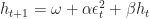
Where h denotes variance, the squared residual, and t the period. The constants must be estimated and updated by the model every period using maximum likelihood. (The explanation for this is beyond the scope of this blog, I recommend using statistical software like R for implementation.) Additionally, one could change the order to change the number of ARCH and GARCH terms included in your model. Sometimes more lags are needed to accurately forecast volatility.

Caution is to be exercised by the user; this is not an end all be all method and it is entirely possible for resulting prediction to be completely different than the true variance. Always check your work and perform diagnostic tests like the Ljung box test to confirm that there is no auto-correlation left in the squared residuals.

Few, it was a long one, I hope that the first part of the post, made the GARCH model more approachable and that this introduction was useful. I encourage you to comment if areas of the post could be made clearer. Finally, stay tuned for part 2 where I am going to give another example of GARCH(1,1) for a value-at-risk estimation (a fairly popular application in academic literature) and part 3 on the EGARCH!

QF

Improved Key Perfomance Statistics

With the goal to improve reader experience on the blog, I will be introducing a new performance statistics report for backtest results. In deciding what I would be using, I used reader feedback and I went on other blogs I follow to see what they were using. This way I think readers will be able to easily compare the different ideas they see across the blogosphere. As a guideline, I will from now on be using a statistical output relatively similar to the output produced by the DVixl platform (highly recommended product). In addition, I am going to be inserting three other measures in the tables. They are described below.

Sortino Ratio

This ratio is a measure of the risk-adjusted return of the strategy. It is, in my opinion an improved version of the popular Sharpe ratio. The Sharpe ratio is computed using the mean return divided by the standard deviation of returns. While its simplicity is appealing, it isn’t a flawless measure (none is); it penalize both upside and downside volatility. From an intuitive point of view, only penalizing downside volatility make more sense, because upside volatility is desirable for investors. This is exactly what the Sortino ratio does (from wiki):

Where R is the asset or portfolio realized return; T is the target or required rate of return for the investment strategy under consideration, (T was originally known as the minimum acceptable return or MAR); DR is the downside risk. Note that for the statistic on the blog, the MAR is going to be 0, same as in the Sharpe calculation.

Historical Value-at-Risk (95%)

For a very nice explanation of the VaR concept, see this article by David Varadi. The value reported will be the ex-post (after the fact) value of the 5th percentile on the negative returns empirical distribution. It indicates that historically, we had daily returns worse that the value 5% of the time. Note that this is a non-parametric VaR which I prefer to the version assuming Gaussian distribution.

I hope that the new format which will be employed in future backtests will satisfy a broader audience of reader, and I also think that it will improve the value of the blog. In a short period of time, I will be posting strategies that I consider more tradable than the concepts I have talked about before and I think that the new format will be better to convey their value.

QF