Basic Introduction to GARCH and EGARCH (part 1)

As request by several readers in light of the previous series of post on using GARCH(1,1) to forecast volatility, here is a very basic introduction post on two models widely used in finance: the GARCH and EGARCH.

One of the great tools of statistics used in finance is the least square model (not exclusively the linear least squares). For the neophyte, the least square model is used to determine the variation of a dependant variable in response to a change in another variable(s) called independent or predictor(s). When we fit a model, the difference between the predicted value and the actual value is called the error term, or residual, it is denoted by the Greek letter epsilon (). As mentioned in one of my all time favorite blog post: Wonder of Residuals by Quantivity, there is a myriad of information and uses to this construct.

When we fit a model, we are, or I am anyway (!), interested in analyzing the size of errors. One of the basic assumptions of the least square model is that the squared error (squared to eliminate the effect of negative numbers) stays constant across every data point in the model. The term used for this equal variance assumption is homoskedasticity. However, with financial time series variance (read volatility or risk) cannot always be assumed constant, browsing through financial data, we can see that some periods are more volatile than others. Keeping this in mind, when fitting a model, this translates to a greater magnitude in the residuals. In addition, these spikes in variance are not randomly placed in time; there is an auto-correlation effect present. In simple terms, we call it volatility clustering, meaning that periods of high variance tend to group up together; think VIX spikes for example. Non-constant variance is referred as heteroskedasticity. This is where the GARCH model comes in, and helps us find a volatility measures that we can use to forecast the residuals in our models and relax the often flawed equal residuals assumption.

Before talking about the GARCH model, I have to quickly introduce its very close cousin, the ARCH (autoregressive conditional heteroskedasticity) model. Consider what must be the easiest way to forecast volatility; the rolling x day standard deviation. Say we look at it on a yearly (252 days) basis. Equipped with the value of this historical standard deviation we want to forecast the value for the next day. Central tendency statistics tells us that the mean is the best guess. I can already hear some of you cringe at the idea.

Using the mean, every 252 observation is equally weighted. However, wouldn’t it make more sense for the more recent observations to weight more? We could perhaps use an exponentially weighted average to solve this problem, but still isn’t the best solution. Another observation could be made about this method; it forgets any data points older than 252 days (their weight is 0). This weighting scheme is not the most desirable for quantitatively oriented investors as they are rather arbitrary. In comes the ARCH model where the weights applied on the residuals are automatically estimated to the best parameters (David Varadi would call it level 1 adaptation). The generalized ARCH model (GARCH) is based on the same principle but with time, the weights get progressively smaller, never reaching 0.

In the previous series of post, I used the GARCH model of order (1,1). Defined like this, the model predicts the period’s variance by looking at the weighted average of the long term historical variance, the predicted variance for the period (second 1, also called the number of GARCH terms) and the previous day squared residual (first 1, also called number of ARCH terms). Or more formally:

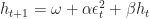
Where h denotes variance, the squared residual, and t the period. The constants must be estimated and updated by the model every period using maximum likelihood. (The explanation for this is beyond the scope of this blog, I recommend using statistical software like R for implementation.) Additionally, one could change the order to change the number of ARCH and GARCH terms included in your model. Sometimes more lags are needed to accurately forecast volatility.

Caution is to be exercised by the user; this is not an end all be all method and it is entirely possible for resulting prediction to be completely different than the true variance. Always check your work and perform diagnostic tests like the Ljung box test to confirm that there is no auto-correlation left in the squared residuals.

Few, it was a long one, I hope that the first part of the post, made the GARCH model more approachable and that this introduction was useful. I encourage you to comment if areas of the post could be made clearer. Finally, stay tuned for part 2 where I am going to give another example of GARCH(1,1) for a value-at-risk estimation (a fairly popular application in academic literature) and part 3 on the EGARCH!

QF